ADCP Example

The following example shows a typical workflow for analyzing ADCP data using DOLfYN’s tools.

A typical ADCP data workflow is broken down into 1. Review the raw data - Check timestamps - Calculate/check that the depth bin locations are correct - Look at velocity, beam amplitude and/or beam correlation data quality 2. Remove data located above the water surface or below the seafloor 3. Check for spurious datapoints and remove if necessary 4. If not already done within the instrument, average the data into bins of a set time length (normally 5 to 10 min) 5. Conduct further analysis as required

Start by importing the necessary DOLfYN tools through MHKiT:

[1]:

# Import core DOLfYN functions
import dolfyn
# Import ADCP-specific API tools
from dolfyn.adp import api

First Steps and QC’ing Data

1.) Set deployment height

Because this is a Nortek instrument, the deployment software doesn’t take into account the deployment height, aka where in the water column the ADCP is. The center of the first depth bin is located at a distance = deployment height + blanking distance + cell size, so the range coordinate needs to be corrected so that ‘0’ corresponds to the seafloor. This can be done in DOLfYN using the set_range_offset function. This same function can be used to account for the depth of a down-facing instrument below the water surface.

Note, if using a Teledyne RDI ADCP, TRDI’s deployment software asks the user to enter the deployment height/depth during configuration. If needed, this can be adjusted after-the-fact using set_range_offset as well.

[5]:

# The ADCP transducers were measured to be 0.6 m from the feet of the lander
api.clean.set_range_offset(ds, 0.6)

So, the center of bin 1 is located at 1.2 m:

[6]:

ds.range

[6]:

<xarray.DataArray 'range' (range: 28)>
array([ 1.2,  1.7,  2.2,  2.7,  3.2,  3.7,  4.2,  4.7,  5.2,  5.7,  6.2,  6.7,
        7.2,  7.7,  8.2,  8.7,  9.2,  9.7, 10.2, 10.7, 11.2, 11.7, 12.2, 12.7,
       13.2, 13.7, 14.2, 14.7])
Coordinates:
  * range    (range) float64 1.2 1.7 2.2 2.7 3.2 ... 12.7 13.2 13.7 14.2 14.7
Attributes:
    units:    m

2.) Remove data beyond surface level

To reduce the amount of data the code must run through, we can remove all data at and above the water surface. Because the instrument was looking up, we can use the pressure sensor data and the function find_surface_from_P. This does require that the pressure sensor was ‘zeroed’ prior to deployment. If the instrument is looking down or lacks pressure data, use the function find_surface to detect the seabed or water surface.

ADCPs don’t measure water salinity, so it will need to be given to the function. The returned dataset contains the an additional variable “depth”. If find_surface_from_P is run after set_range_offset, depth is the distance of the water surface away from the seafloor; otherwise it is the distance to the ADCP pressure sensor.

After calculating depth, data in depth bins at and above the physical water surface can be removed using nan_beyond_surface. Note that this function returns a new dataset.

[7]:

api.clean.find_surface_from_P(ds, salinity=31)
ds = api.clean.nan_beyond_surface(ds)

3.) Correlation filter

Once beyond-surface bins have been removed, ADCP data is typically filtered by acoustic signal correlation to clear out spurious velocity datapoints (caused by bubbles, kelp, fish, etc moving through one or multiple beams).

We can take a quick look at the data to see about where this value should be using xarray’s built-in plotting. In the following line of code, we use xarray’s slicing capabilities to show data from beam 1 between a range of 0 to 10 m from the ADCP.

Not all ADCPs return acoustic signal correlation, which in essence is a quantitative measure of signal quality. ADCPs with older hardware do not provide a correlation measurement, so this step will be skipped with these instruments.

[8]:

%matplotlib inline
ds['corr'].sel(beam=1, range=slice(0,10)).plot()

[8]:

<matplotlib.collections.QuadMesh at 0x22bc6980cd0>

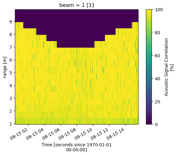
It’s a good idea to check the other beams as well. Much of this data is high quality, and to not lose data will low correlation caused by natural variation, we’ll use the correlation_filter to set velocity values corresponding to correlations below 50% to NaN.

Note that this threshold is dependent on the deployment environment and instrument, and it isn’t uncommon to use a value as low as 30%, or to pass on this function completely.

[9]:

ds = api.clean.correlation_filter(ds, thresh=50)

Review the Data

Now that the data has been cleaned, the next step is to rotate the velocity data into true East, North, Up coordinates.

ADCPs use an internal compass or magnetometer to determine magnetic ENU directions. The set_declination function takes the user supplied magnetic declination (which can be looked up online for specific coordinates) and adjusts the velocity data accordingly.

Instruments save vector data in the coordinate system specified in the deployment configuration file. To make the data useful, it must be rotated through coordinate systems (“beam”<->”inst”<->”earth”<->”principal”), done through the rotate2 function. If the “earth” (ENU) coordinate system is specified, DOLfYN will automatically rotate the dataset through the necessary coordinate systems to get there. The inplace set as true will alter the input dataset “in place”, a.k.a. it not create a new dataset.

Because this ADCP data was already in the “earth” coordinate system, rotate2 will return the input dataset. set_declination will run correctly no matter the coordinate system.

[10]:

dolfyn.set_declination(ds, declin=15.8, inplace=True) # 15.8 deg East
dolfyn.rotate2(ds, 'earth', inplace=True)

Data is already in the earth coordinate system

To rotate into the principal frame of reference (streamwise, cross-stream, vertical), if desired, we must first calculate the depth-averaged principal flow heading and add it to the dataset attributes. Then the dataset can be rotated using the same rotate2 function. We use inplace=False because we do not want to alter the input dataset.

[11]:

ds.attrs['principal_heading'] = dolfyn.calc_principal_heading(ds['vel'].mean('range'))
ds_streamwise = dolfyn.rotate2(ds, 'principal', inplace=False)

Because this deployment was set up in “burst mode”, the next standard step in this analysis is to average the velocity data into time bins.

If an instrument was set up to record velocity data in an “averaging mode” (a specific profile and/or average interval, e.g. take 5 minutes of data every 30 minutes), this step was completed within the ADCP during deployment and can be skipped.

To average the data into time bins (aka ensembles), start by initiating the binning tool VelBinner. “n_bin” is the number of data points in each ensemble, in this case 300 seconds worth of data, and “fs” is the sampling frequency, which is 1 Hz for this deployment. Once initiated, average the data into ensembles using the binning tool’s do_avg function.

[12]:

avg_tool = api.VelBinner(n_bin=ds.fs*300, fs=ds.fs)
ds_avg = avg_tool.do_avg(ds)

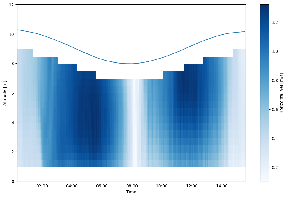
Two more variables not automatically provided that may be of interest are the horizontal velocity magnitude (speed) and its direction, respectively U_mag and U_dir. There are included as “shortcut” functions, and are accessed through the keyword velds, as shown in the code block below. The full list of “shorcuts” are listed here.

[13]:

ds_avg['U_mag'] = ds_avg.velds.U_mag
ds_avg['U_dir'] = ds_avg.velds.U_dir

Plotting can be accomplished through the user’s preferred package. Matplotlib is shown here for simplicity, and flow speed and direction are plotted below with a blue line delineating the water surface level.

[14]:

%matplotlib inline
from matplotlib import pyplot as plt
import matplotlib.dates as dt

ax = plt.figure(figsize=(12,8)).add_axes([.14, .14, .8, .74])
# Plot flow speed
t = dolfyn.time.dt642date(ds_avg.time)
plt.pcolormesh(t, ds_avg['range'], ds_avg['U_mag'], cmap='Blues', shading='nearest')
# Plot the water surface
ax.plot(t, ds_avg['depth'])

# Set up time on x-axis
ax.set_xlabel('Time')
ax.xaxis.set_major_formatter(dt.DateFormatter('%H:%M'))

ax.set_ylabel('Altitude [m]')
ax.set_ylim([0, 12])
plt.colorbar(label='Horizontal Vel [m/s]')

[14]:

<matplotlib.colorbar.Colorbar at 0x22bc076b3a0>

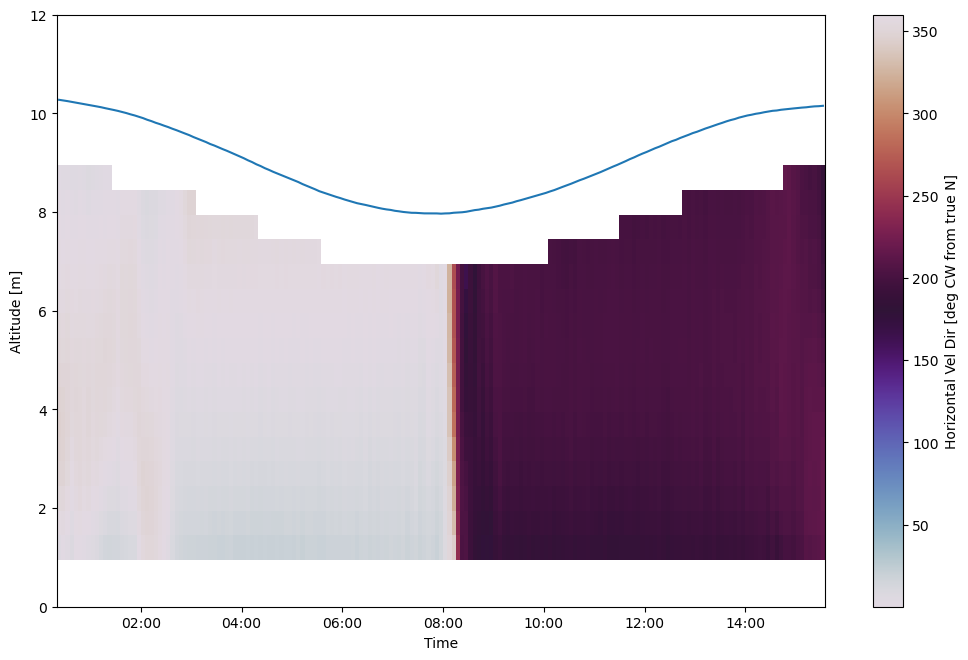
[15]:

ax = plt.figure(figsize=(12,8)).add_axes([.14, .14, .8, .74])
# Plot flow direction
plt.pcolormesh(t, ds_avg['range'], ds_avg['U_dir'], cmap='twilight', shading='nearest')
# Plot the water surface
ax.plot(t, ds_avg['depth'])

# set up time on x-axis
ax.set_xlabel('Time')
ax.xaxis.set_major_formatter(dt.DateFormatter('%H:%M'))

ax.set_ylabel('Altitude [m]')
ax.set_ylim([0, 12])
plt.colorbar(label='Horizontal Vel Dir [deg CW from true N]')

[15]:

<matplotlib.colorbar.Colorbar at 0x22bc6204190>

Saving and Loading DOLfYN datasets

Datasets can be saved and reloaded using the save and load functions. Xarray is saved natively in netCDF format, hence the “.nc” extension.

Note: DOLfYN datasets cannot be saved using xarray’s native ds.to_netcdf; however, DOLfYN datasets can be opened using xarray.open_dataset.

[16]:

# Uncomment these lines to save and load to your current working directory
#dolfyn.save(ds, 'your_data.nc')
#ds_saved = dolfyn.load('your_data.nc')