Motion Correction

The Nortek Vector ADV can be purchased with an Inertial Motion Unit (IMU) that measures the ADV motion. These measurements can be used to remove motion from ADV velocity measurements when the ADV is mounted on a moving platform (e.g. a mooring). This approach has been found to be effective for removing high-frequency motion from ADV measurements, but cannot remove low-frequency ($\lesssim$ 0.03Hz) motion because of bias-drift inherent in IMU accelerometer sensors that contaminates motion estimates at those frequencies.

This documentation is designed to document the methods for performing motion correction of ADV-IMU measurements. The accuracy and applicability of these measurements is beyond the scope of this documentation (see [Harding_etal_2017], [Kilcher_etal_2017]).

Nortek’s Signature ADCP’s are now also available with an Altitude and Heading Reference System (AHRS), but DOLfYN does not yet support motion correction of ADCP data.

Pre-Deployment Requirements

In order to perform motion correction the ADV-IMU must be assembled and configured correctly:

The ADV head must be rigidly connected to the ADV pressure case.
The ADV software must be configured properly. In the ‘Deployment Planning’ frame of the Vector Nortek Software, be sure that:
1. The IMU sensor is enabled (checkbox) and set to record ‘dAng dVel Orient’.
2. The ‘Coordinate system’ must be set to ‘XYZ’.
3. It is recommended to set the ADV velocity range to ± 4 m/s, or larger.
For cable-head ADVs be sure to record the position and orientation of the ADV head relative to the ADV pressure case ‘inst’ coordinate system (Figure 1). This information is specified in terms of the following variables:
inst2head_rotmat
The rotation matrix (a 3-by-3 array) that rotates vectors in the ‘inst’ coordinate system, to the ADV ‘head’ coordinate system. For fixed-head ADVs this is the identity matrix, but for cable-head ADVs it is an arbitrary unimodular (determinant of 1) matrix. This property must be in dat.data_vars in order to do motion correction.

inst2head_vec
The 3-element vector that specifies the position of the ADV head in the inst coordinate system (IMU coordinate system, Figure 1). This property must be in dat.attrs in order to do motion correction.

These variables are set in either the userdata.json file (prior to calling
dolfyn.read), or by setting them explicitly after the data file has been read:
dat.velds.set_inst2head_rotmat(<3x3 rotation matrix>) dat.attrs['inst2head_vec'] = np.array([3-element vector])

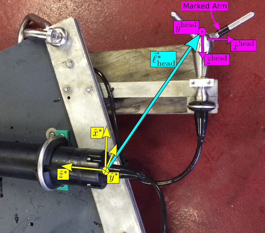
ADV head and inst coordinate systems. — Figure 1 The ADV ‘inst’ (yellow) and head (magenta) coordinate systems. The $\hat{x}^\mathrm{head}$ -direction is known by the black-band around the transducer arm, and the $\hat{x}^*$ -direction is marked by a notch on the end-cap (indiscernible in the image). The cyan arrow indicates the `inst2head_vec` vector $\vec{\ell}_{head}^*$ . The perspective slightly distorts the fact that $\hat{x}^\mathrm{head} \parallel - \hat{z}^*$ , $\hat{y}^\mathrm{head} \parallel -\hat{y}^*$ , and $\hat{z}^\mathrm{head} \parallel -\hat{x}^*$ .

Specify metadata in a JSON file

The values in dat.attrs can also be set in a json file, <data_filename>.userdata.json, containing a single json-object. For example, the contents of these files should look something like:

{"inst2head_rotmat": "identity",
 "inst2head_vec": [-1.0, 0.5, 0.2],
 "motion accel_filtfreq Hz": 0.03,
 "declination": 8.28,
 "latlon": [39.9402, -105.2283]
}

Prior to reading a binary data file my_data.VEC, you can create a my_data.userdata.json file. Then when you do dolfyn.read('my_data.VEC'), DOLfYN will read the contents of my_data.userdata.json and include that information in the dat.attrs attribute of the returned data object. This feature is provided so that meta-data can live alongside your binary data files.

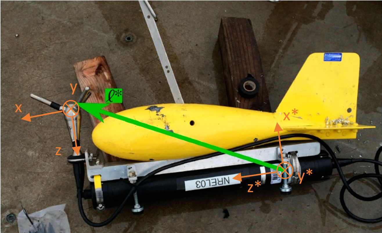
Figure 2 ADV mounted on a Columbus-type sounding weight.

The ‘userdata.json’ file corresponding to the ADV sounding weight in Figure 2 looks like:

{"inst2head_rotmat": [[ 0, 0,-1],
                      [ 0, 1, 0],
                      [ 1, 0, 0]],
 "inst2head_vec": [0.04, 0, 0.20],
 "motion accel_filtfreq Hz": 0.03,
}

Data Processing

After making ADV-IMU measurements, the DOLfYN package can perform motion correction processing steps on the ADV data. Assuming you have created a vector_data_imu.userdata.json file (to go with your vector_data_imu.vec data file), motion correction is fairly simple. You can either:

Utilize the DOLfYN API to perform motion-correction explicitly in Python:

import dolfyn.adv.api as avm

Load your data file, for example:

dat = avm.read('vector_data_imu01.vec')

Then perform motion correction:

avm.correct_motion(dat, accel_filtfreq=0.1) # specify the filter frequency in Hz.

For users who want to perform motion correction with minimal Python scripting, the motcorrect_vector.py script can be used. So long as DOLfYN has been installed properly, you can use this script from the command line in a directory which contains your data files:
```
$ python motcorrect_vector.py vector_data_imu01.vec
```
By default this will write a Matlab file containing your motion-corrected ADV data in ENU coordinates. Note that for fixed-head ADVs (no cable b/t head and battery case), the standard values for inst2head_rotmat and inst2head_vec can be specified by using the --fixed-head command-line parameter:
```
$ python motcorrect_vector.py --fixed-head vector_data_imu01.vec
```
Otherwise, these parameters should be specified in the .userdata.json file, as described above.

The motcorrect_vector.py script also allows the user to specify the accel_filtfreq using the -f flag. Therefore, to use a filter frequency of 0.1Hz (as opposed to the default 0.033Hz), you could do:
```
$ python motcorrect_vector.py -f 0.1 vector_data_imu01.vec
```
It is also possible to do motion correction of multiple data files at once, for example:
```
$ python motcorrect_vector.py vector_data_imu01.vec vector_data_imu02.vec
```
In all of these cases the script will perform motion correction on the specified file and save the data in ENU coordinates, in Matlab format. Happy motion-correcting!

After following one of these paths, your data will be motion corrected and its .u, .v and .w attributes are in an East, North and Up (ENU) coordinate system, respectively. In fact, all vector quantities in dat are now in this ENU coordinate system. See the documentation of the correct_motion() function for more information.

A key input parameter of motion-correction is the high-pass filter frequency that removes low-frequency bias drift from the IMU accelerometer signal (the default value is 0.03 Hz, a ~30 second period). For more details on choosing the appropriate value for a particular application, please see [Kilcher_etal_2016].

[Kilcher_etal_2016]

Kilcher, L.; Thomson, J.; Talbert, J.; DeKlerk, A.; 2016, “Measuring Turbulence from Moored Acoustic Doppler Velocimeters” National Renewable Energy Lab, Report Number 62979.

[Harding_etal_2017]

Harding, S., Kilcher, L., Thomson, J. (2017). Turbulence Measurements from Compliant Moorings. Part I: Motion Characterization. Journal of Atmospheric and Oceanic Technology, 34(6), 1235-1247. doi: 10.1175/JTECH-D-16-0189.1

[Kilcher_etal_2017]

Kilcher, L., Thomson, J., Harding, S., & Nylund, S. (2017). Turbulence Measurements from Compliant Moorings. Part II: Motion Correction. Journal of Atmospheric and Oceanic Technology, 34(6), 1249-1266. doi: 10.1175/JTECH-D-16-0213.1

Motion Correction Examples

The two following examples depict the standard workflow for analyzing ADV-IMU data using DOLfYN.

ADV Motion Correction Ex.1

# To get started first import the DOLfYN ADV advanced programming
# interface (API):
import dolfyn.adv.api as api
from dolfyn import time

# Import matplotlib tools for plotting the data:
from matplotlib import pyplot as plt
import matplotlib.dates as dt
from datetime import datetime
import numpy as np

##############################
# User input and customization

# The file to load:
fname = '../../dolfyn/example_data/vector_data_imu01.vec'

# This is the vector from the ADV head to the instrument frame, in meters,
# in the ADV coordinate system.
inst2head_vec = np.array([0.48, -0.07, -0.27])

# This is the orientation matrix of the ADV head relative to the body
# (battery case).
# In this case the head was aligned with the body, so it is the
# identity matrix:
inst2head_rotmat = np.eye(3)

# The time range of interest.
# The instrument was in place on the seafloor starting at 12:08:30 on June 12, 2012.
t_range = [time.date2dt64(datetime(2012, 6, 12, 12, 8, 30)),
           # The data is good to the end of the file.
           time.date2dt64(datetime(2012, 6, 13))]

# This is the filter to use for motion correction:
accel_filter = 0.1

# End user input section.
###############################

# Read a file containing adv data:
dat_raw = api.read(fname, userdata=False)

# Crop the data for t_range
t_range_inds = (t_range[0] < dat_raw.time) & (dat_raw.time < t_range[1])
dat = dat_raw.isel(time=t_range_inds)

# Set the inst2head rotation matrix and vector
api.set_inst2head_rotmat(dat, inst2head_rotmat)
dat.attrs['inst2head_vec'] = inst2head_vec

# Then clean the file using the Goring+Nikora method:
mask = api.clean.GN2002(dat.vel)
dat['vel'] = api.clean.clean_fill(dat.vel, mask, method='cubic')

####
# Create a figure for comparing screened data to the original.
fig = plt.figure(1, figsize=[8, 4])
fig.clf()
ax = fig.add_axes([.14, .14, .8, .74])

# Plot the raw (unscreened) data:
ax.plot(dat_raw.time, dat_raw.velds.u, 'r-', rasterized=True)

# Plot the screened data:
ax.plot(dat.time, dat.velds.u, 'g-', rasterized=True)
bads = np.abs(dat.velds.u - dat_raw.velds.u.isel(time=t_range_inds))
ax.text(0.55, 0.95,
        "%0.2f%% of the data were 'cleaned'\nby the Goring and Nikora method."
        % (float(sum(bads > 0)) / len(bads) * 100),
        transform=ax.transAxes,
        va='top',
        ha='left')

# Add some annotations:
text0 = dt.date2num(datetime(2012, 6, 12, 12, 8, 30))
ax.axvspan(dt.date2num(datetime(2012, 6, 12, 12)),
           text0, zorder=-10, facecolor='0.9',
           edgecolor='none')
ax.text(0.13, 0.9, 'Mooring falling\ntoward seafloor',
        ha='center', va='top', transform=ax.transAxes,
        size='small')
ax.text(text0 + 0.0001, 0.6, 'Mooring on seafloor',
        size='small',
        ha='left')
ax.annotate('', (text0 + 0.006, 0.3),
            (text0, 0.3),
            arrowprops=dict(facecolor='black', shrink=0.0),
            ha='right')

# Finalize the figure
# Format the time axis:
tkr = dt.MinuteLocator(interval=5)
frmt = dt.DateFormatter('%H:%M')
ax.xaxis.set_major_locator(tkr)
ax.xaxis.set_minor_locator(dt.MinuteLocator(interval=1))
ax.xaxis.set_major_formatter(frmt)
ax.set_ylim([-3, 3])

# Label the axes:
ax.set_ylabel('$u\,\mathrm{[m/s]}$', size='large')
ax.set_xlabel('Time [June 12, 2012]')
ax.set_title('Data cropping and cleaning')
ax.set_xlim([dt.date2num(datetime(2012, 6, 12, 12)),
             dt.date2num(datetime(2012, 6, 12, 12, 30))])
####

dat_cln = dat.copy(deep=True)

# Perform motion correction (including rotation into earth frame):
dat = api.correct_motion(dat, accel_filter)

# Rotate the uncorrected data into the earth frame,
# for comparison to motion correction:
api.rotate2(dat_cln, 'earth')

# Then rotate it into a 'principal axes frame':
dat.attrs['principal_heading'] = api.calc_principal_heading(dat.vel)
dat_cln.attrs['principal_heading'] = api.calc_principal_heading(dat_cln.vel)
api.rotate2(dat, 'principal')
api.rotate2(dat_cln, 'principal')

# Average the data and compute turbulence statistics
dat_bin = api.calc_turbulence(dat, n_bin=9600, fs=dat.fs, n_fft=4096)
dat_cln_bin = api.calc_turbulence(
    dat_cln, n_bin=9600, fs=dat_cln.fs, n_fft=4096)

####
# Figure to look at spectra
fig2 = plt.figure(2, figsize=[6, 6])
fig2.clf()
ax = fig2.add_axes([.14, .14, .8, .74])

ax.loglog(dat_bin.freq, dat_bin['psd'].sel(S='Sxx').mean(axis=0),
          'b-', label='motion corrected')
ax.loglog(dat_cln_bin.freq, dat_cln_bin['psd'].sel(S='Sxx').mean(axis=0),
          'r-', label='no motion correction')

# Add some annotations
ax.axhline(1.7e-4, color='k', zorder=21)
ax.text(2e-3, 1.7e-4, 'Doppler noise level', va='bottom', ha='left',)

ax.text(1, 2e-2, 'Motion\nCorrection')
ax.annotate('', (3.6e-1, 3e-3), (1, 2e-2),
            arrowprops={'arrowstyle': 'fancy',
                        'connectionstyle': 'arc3,rad=0.2',
                        'facecolor': '0.8',
                        'edgecolor': '0.6'},
            ha='center')

ax.annotate('', (1.6e-1, 7e-3), (1, 2e-2),
            arrowprops={'arrowstyle': 'fancy',
                        'connectionstyle': 'arc3,rad=0.2',
                        'facecolor': '0.8',
                        'edgecolor': '0.6'},
            ha='center')

# Finalize the figure
ax.set_xlim([1e-3, 20])
ax.set_ylim([1e-4, 1])
ax.set_xlabel('frequency [hz]')
ax.set_ylabel('$\mathrm{[m^2s^{-2}/hz]}$', size='large')

f_tmp = np.logspace(-3, 1)
ax.plot(f_tmp, 4e-5 * f_tmp ** (-5. / 3), 'k--')

ax.set_title('Velocity Spectra')
ax.legend()
ax.axvspan(1, 16, 0, .2, facecolor='0.8', zorder=-10, edgecolor='none')
ax.text(4, 4e-4, 'Doppler noise', va='bottom', ha='center',
        #bbox=dict(facecolor='w', alpha=0.9, edgecolor='none'),
        zorder=20)

ADV Motion Correction Ex.2

import dolfyn
import dolfyn.adv.api as api

import numpy as np
from datetime import datetime
import matplotlib.pyplot as plt
import matplotlib.dates as mpldt


##############################################################################
# User-input data
fname = '../../dolfyn/example_data/vector_data_imu01.VEC'
accel_filter = .03  # motion correction filter [Hz]
ensemble_size = 32*300  # sampling frequency * 300 seconds

# Read the data in, use the '.userdata.json' file
data_raw = dolfyn.read(fname, userdata=True)

# Crop the data for the time range of interest:
t_start = dolfyn.time.date2dt64(datetime(2012, 6, 12, 12, 8, 30))
t_end = data_raw.time[-1]
data = data_raw.sel(time=slice(t_start, t_end))


##############################################################################
# Clean the file using the Goring, Nikora 2002 method:
bad = api.clean.GN2002(data.vel)
data['vel'] = api.clean.clean_fill(data.vel, bad, method='cubic')
# To not replace data:
# data.coords['mask'] = (('dir','time'), ~bad)
# data.vel.values = data.vel.where(data.mask)

# plotting raw vs qc'd data
ax = plt.figure(figsize=(20, 10)).add_axes([.14, .14, .8, .74])
ax.plot(data_raw.time, data_raw.velds.u, label='raw data')
ax.plot(data.time, data.velds.u, label='despiked')
ax.set_xlabel('Time')
ax.xaxis.set_major_formatter(mpldt.DateFormatter('%D %H:%M'))
ax.set_ylabel('u-dir velocity, (m/s)')
ax.set_title('Raw vs Despiked Data')
plt.legend(loc='upper right')
plt.show()

data_cleaned = data.copy(deep=True)


##############################################################################
# Perform motion correction
data = api.correct_motion(data, accel_filter, to_earth=False)
# For reference, dolfyn defines ‘inst’ as the IMU frame of reference, not
# the ADV sensor head
# After motion correction, the pre- and post-correction datasets coordinates
# may not align. Since here the ADV sensor head and battery body axes are
# aligned, data.u is the same axis as data_cleaned.u

# Plotting corrected vs uncorrect velocity in instrument coordinates
ax = plt.figure(figsize=(20, 10)).add_axes([.14, .14, .8, .74])
ax.plot(data_cleaned.time, data_cleaned.velds.u, 'g-', label='uncorrected')
ax.plot(data.time, data.velds.u, 'b-', label='motion-corrected')
ax.set_xlabel('Time')
ax.xaxis.set_major_formatter(mpldt.DateFormatter('%D %H:%M'))
ax.set_ylabel('u velocity, (m/s)')
ax.set_title('Pre- and Post- Motion Corrected Data in XYZ coordinates')
plt.legend(loc='upper right')
plt.show()


# Rotate the uncorrected data into the earth frame for comparison to motion
# correction:
dolfyn.rotate2(data, 'earth', inplace=True)
data_uncorrected = dolfyn.rotate2(data_cleaned, 'earth', inplace=False)

# Calc principal heading (from earth coordinates) and rotate into the
# principal axes
data.attrs['principal_heading'] = dolfyn.calc_principal_heading(data.vel)
data_uncorrected.attrs['principal_heading'] = dolfyn.calc_principal_heading(
    data_uncorrected.vel)
data.velds.rotate2('principal')
data_uncorrected.velds.rotate2('principal')

# Plotting corrected vs uncorrected velocity in principal coordinates
ax = plt.figure(figsize=(20, 10)).add_axes([.14, .14, .8, .74])
ax.plot(data_uncorrected.time, data_uncorrected.velds.u,
        'g-', label='uncorrected')
ax.plot(data.time, data.velds.u, 'b-', label='motion-corrected')
ax.set_xlabel('Time')
ax.xaxis.set_major_formatter(mpldt.DateFormatter('%D %H:%M'))
ax.set_ylabel('streamwise velocity, (m/s)')
ax.set_title('Corrected and Uncorrected Data in Principal Coordinates')
plt.legend(loc='upper right')
plt.show()


##############################################################################
# Create velocity spectra
# Initiate tool to bin data based on the ensemble length. If n_fft is none,
# n_fft is equal to n_bin
ensemble_tool = api.ADVBinner(n_bin=9600, fs=data.fs, n_fft=4800)

# motion corrected data
mc_spec = ensemble_tool.calc_psd(data.vel, freq_units='Hz')
# not-motion corrected data
unm_spec = ensemble_tool.calc_psd(data_uncorrected.vel, freq_units='Hz')
# Find motion spectra from IMU velocity
uh_spec = ensemble_tool.calc_psd(data['velacc'] + data['velrot'],
                                 freq_units='Hz')

# Plot U, V, W spectra
U = ['u', 'v', 'w']
for i in range(len(U)):
    plt.figure(figsize=(15, 13))
    plt.loglog(uh_spec.freq, uh_spec[i].mean(axis=0), 'c',
               label=('motion spectra ' + str(accel_filter) + 'Hz filter'))
    plt.loglog(unm_spec.freq, unm_spec[i].mean(
        axis=0), 'r', label='uncorrected')
    plt.loglog(mc_spec.freq, mc_spec[i].mean(
        axis=0), 'b', label='motion corrected')

    # plot -5/3 slope
    f_tmp = np.logspace(-2, 1)
    plt.plot(f_tmp, 4e-5*f_tmp**(-5/3), 'k--', label='f^-5/3 slope')

    if U[i] == 'u':
        plt.title('Spectra in streamwise dir')
    elif U[i] == 'v':
        plt.title('Spectra in cross-stream dir')
    else:
        plt.title('Spectra in up dir')
    plt.xlabel('Freq [Hz]')
    plt.ylabel('$\mathrm{[m^2s^{-2}/Hz]}$', size='large')
    plt.legend()
plt.show()